Optimization Algorithms in Deep Learning

We use optimization algorithms to update parameters of a model so that they minimize a loss function.

Gradient Descent and Stochastic Gradient Descent

Gradient Descent is an iterative process to minimize a function. Basically the key idea is to update the function in the opposite direction of the gradient.

In a ML setting, you compute the gradients across the entire dataset and then update the parameters. However, in most cases, the dataset would be too big. Hence, we use Stochastic Gradient Descent.

In SGD, the gradient is calculated for each training datapoint or a batch of them, which is then used to update the function. However, what's the guarantee that this would converge to the same result as Gradient Descent? How does calculating gradient on small batches of data would give us the same gradient as that of the entire dataset?

Apparently it does and it is proved in [1],

Robbins-Monro Algorithm

The algorithm addresses the problem - "How do you find a root of an equation when you cannot observe the equation directly?"

Given
$x_{n}$ - The current estimate of the root
$y_{n}$ - The noisy observation of the function taken at $x_{n}$
$t$ - The target value for the function (In most cases it is 0)
$α$ - The Learning Rate

Then

x_{n + 1} = x_{n} - α (y_{n} - t)

As long as the learning rate follows few conditions, then eventually $x_{n}$ will converge to the true value of the parameters that gives the target value. If the target value is 0, our function is the gradient of the model and the noisy observation is the value of the gradient of the loss function we get based on a small batch of training data, then we can see that this resembles the familiar update equation.

The Conditions of the Learning Rate are as follows:

\sum_{1}^{\infty} α = \infty

\sum_{1}^{\infty} α^{2} < \infty

The Issue with SGD - Pathological Curvature

Pasted image 20251121222342.png
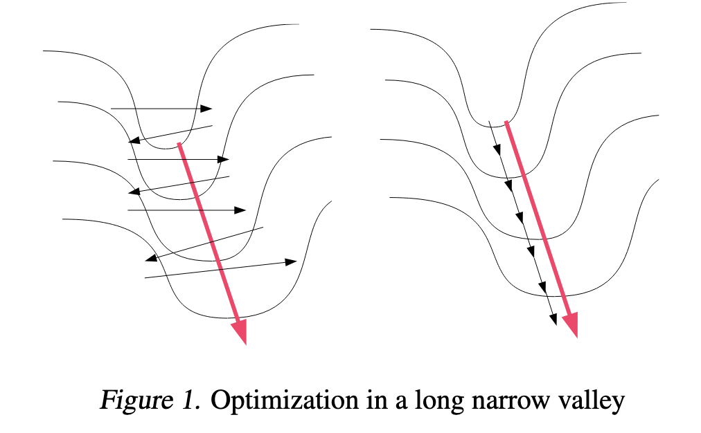
(Image taken from [2])
Pathological Curvature - Gradient is high in a direction and low in the another and the minima is present in the direction where the gradient is low.

Given we have the curvature as shown above, Gradient Descent would follow the black lines on the left, while the ideal path would be the red line. This is just ineffective.

Using Hessian were one of the first approaches, then came the Newton method. However, I am not going to be talking about them for now. (P.S They are a talk for another day)

So how do you solve this?

Adding Momentum

By looking at the path taken by Gradient Descent, an intuitive way would be include the past gradient information. That's exactly momentum.

The Classical Momentum Method is as follows
Given an objective function $f (θ)$ to be minimized,

v_{t + 1} = μ v_{t} - ϵ \nabla f (θ_{t})

θ_{t + 1} = θ_{t} + v_{t + 1}

$v$ is the momentum and it stores the gradient data across iterations.
$μ$ is the momentum co-efficient.

The gradient doesn't change a lot in the directions of low gradient values (Note: Look at the Image earlier) while, they change and cancel out in the high gradient areas. This ensures that the gradient from the low-curvature areas persist and be amplified by momentum.

Math Notation - Condition Number of a Curvature - Ratio of the largest and smallest values of the Hessian Matrix at a specific point

Given R is the condition number of the curvature at the minimum, then [3] showed that Classical Momentum requires $\sqrt{R}$ times fewer iterations compared to Gradient Descent, if we have the correct value for $μ$ . $μ$ should be set to $(\sqrt{R} - 1) / (\sqrt{R} + 1)$ .

NAG - Nesterov's Accelerated Gradient

It is a tiny change to the classical momentum. Instead of calculating the momentum from the current position, it adds a lookahead. It calculates the momentum with the following formula

v_{t + 1} = μ v_{t} - ϵ \nabla f (θ_{t} + μ v_{t})

θ_{t + 1} = θ_{t} + v_{t + 1}

While Momentum was helpful in fixing the direction of each step, there have been approaches dealing with the size of each step.

Adagrad

Introduced in [4]

Momentum based methods and SGD sets a uniform global learning rate for all the parameters.

However, in ML, you try to learn a lot from infrequent phenomena and try to reduce the importance of frequent and common phenomena. Similarly, we want to give a higher weight to updated made to less frequently updated parameters compared to the frequently updated parameters.

AdaGrad achieves it as follows:

θ_{t + 1} = θ_{t} - \frac{η}{\sqrt{v + ϵ}} g_{t}

$v$ is the sum of squared gradients.

This introduces the issue of the sum of squared gradients exploding.

RMSprop

Instead of just storing the sum of squared gradients, Introduce decay so that it doesn't explode.

In RMSprop, G is defined as follows:

v_{t} = β v_{t - 1} + (1 - β) . g_{t}^{2}

Adam and a variant of it called AdamW are the popular choices for optimizations. They store two exponential moving averages of variables, one for the past gradients (momentum) and another for the square of the gradients. The update to the parameters is a scaled version of the first moving average (momentum). It is scaled using the second moving average. However, this uses a lot of memory.

The update matrices produced by Adam and SGD are low-rank matrices, meaning updates are being dominated by a few directions. This makes it difficult to learn the rare directions.

Adam

Adaptive Moment Estimation - Adam

Introduced in [5]

It combines the ideas of both the approaches and deals with both the direction and magnitude of the step.

Algorithm

The Algorithm is as follows
Given
$α$ - Stepsize
$β_{1}, β_{2} \in [0, 1)$ - Exponential Decay Rates for the Moment Estimates
$f (θ)$ - Objective Function
$θ_{0}$ - Initial Parameter Vector

Initialize $m_{0}$ and $v_{0}$ to 0, where $m$ and $v$ represent the first and second moments.
Then for each iteration do the following
1. Get the gradients
$g_{t} = \nabla_{θ} f_{t} (θ_{t - 1})$
1. Update the first moment
$m_{t} = β_{1} m_{t - 1} + (1 - β_{1}) g_{t}$
1. Update the second moment
$v_{t} = β_{2} v_{t - 1} + (1 - β_{2}) g_{t}^{2}$
1. Compute bias correction terms
${\hat{m}}_{t} = m_{t} / (1 - β_{1}^{t})$ ${\hat{v}}_{t} = v_{t} / (1 - β_{2}^{t})$
1. Update Parameters
$θ_{t} = θ_{t - 1} - α {\hat{m}}_{t} / (\sqrt{\hat{v}} + ϵ)$

Why Adam and why not just RMSprop with Momentum?

We could just combine RMSprop with momentum and call it a day. Why do we need Adam?

In both of the methods, we initialize the moments to zero. This causes an initialization bias. Due to exponential averaging, the zero initialization causes the step sizes to be very small at the start.

However, in the case of Adam, the bias correction terms saves it. In the early training steps, due to the high values of $β_{1}$ and $β_{2}$ , we scale the values up. Then in the later training steps, $β_{1}^{t}$ and $β_{2}^{t}$ will be low, thus disappearing.

How do you do Weight Decay in Adam?

Before Adam, L2 Regularization was used as a replacement for Weight Decay. This replacement works well with SGD but it doesn't fit right with Adam.

The Penalty term of L2 Regularization gets added to the gradient and this causes the weights to have different rates of decay based on their variance.

However, we would like to have uniform decay as a means of regularization.

So instead of adding the penalty term while calculating gradients, instead add it at the time of updating parameters as a separate term.

This is the idea behind AdamW, introduced in [6]

Muon

Muon - MomentUm Orthogonalized by Newton-Schulz

It is an optimizer used specifically for 2D weights, as seen in the case of Linear layers.

The Muon Update could be written as follows:

W_{t + 1} = W_{t} - α \sqrt{\frac{f a n - o u t}{f a n - i n}} N e w t o n S c h u l z (\nabla_{W} L)

We want the updates to the weight to cause a bounded change to the outputs. We could write it formally as minimize the loss while maintaining a bound on the outputs.

Assuming that $y$ is the outputs of our model, we have

m i n_{Δ W} (\nabla_{W} L, Δ W) subject to | | Δ y | |_{R M S} \leq K

where $K$ is just a constant

How do you go from a bound on the outputs to a bound on the weights?

So, for a linear layer

Δ y = (W + Δ W) x - W x = Δ W

| | Δ y | |_{R M S} = | | Δ W x | |_{R M S}

So, An operator norm of a matrix tells how much it can stretch an input vector.

RMS-to-RMS operator norm gives the maximum amount by which a matrix can increase the average size of its inputs.

| | W | |_{R M S - > R M S} = m a x_{x \neq 0} \frac{| | W_{x} | |_{R M S}}{| | x | |_{R M S}}

We can write it using the spectral norm as well. Spectral Norm refers to the largest singular value in a matrix.

| | W | |_{R M S - > R M S} = \sqrt{\frac{f a n - o u t}{f a n - i n}} | | W | |_{*}

where $| | W | |_{*}$ is the spectral norm.

Substituting this in place of the bound

(Note: Spectral Norm is a whole lot more interesting - https://atom-101.github.io/blog/posts/2022-03-18-spectral-norm.html)

Coming back to the bound on the outputs, we could say

| | Δ y | | \leq | | Δ W | |_{R M S - > R M S} | | x | |_{R M S}

So,

m i n_{Δ W} (\nabla_{W} L, Δ W) subject to | | Δ W | |_{R M S - > R M S} \leq K

Assuming the Gradient has a SVD given by $U \sum V^{T}$ , the solution to the above bound is

Δ W = - K * \sqrt{\frac{f a n - o u t}{f a n - i n}} U V^{T}

$U V^{T}$ could be seen as the orthogonalizing the gradient. However, we can't perform SVD at scale efficiently. How do you perform orthogonalization efficiently? That is Newton Schulz Matrix iteration.

I will write a separate blog about Newton Schulz Matrix Iteration.

Note - It optimizes 2D parameters, we can convert convolutional weights to 2D params to use Muon for them as well.

References

[1]

H. Robbins and S. Monro, “A Stochastic Approximation Method,” The Annals of Mathematical Statistics, vol. 22, no. 3, pp. 400–407, Sep. 1951, doi: 10.1214/aoms/1177729586.

[2]

J. Martens, “Deep learning via Hessian-free optimization,” in Proceedings of the 27th International Conference on International Conference on Machine Learning, in ICML’10. Madison, WI, USA: Omnipress, Jun. 2010, pp. 735–742.

[3]

B. T. Polyak, “Some methods of speeding up the convergence of iteration methods,” USSR Computational Mathematics and Mathematical Physics, vol. 4, no. 5, pp. 1–17, Jan. 1964, doi: 10.1016/0041-5553(64)90137-5.

[4]

Duchi, John, Elad Hazan, and Yoram Singer. "Adaptive subgradient methods for online learning and stochastic optimization." Journal of machine learning research 12.7 (2011)

[5]

Kingma, Diederik P. "Adam: A method for stochastic optimization." arXiv preprint arXiv:1412.6980 (2014).

[6]

Loshchilov, Ilya, and Frank Hutter. "Decoupled weight decay regularization." arXiv preprint arXiv:1711.05101 (2017).